week 1 - Probability and Statistics for Business - I
week 1
1. Statistic categorization
categorized into two main parts
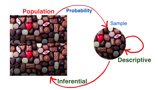
- Descriptive statistics
- Inferential statistics
1.1 Descriptive statistics
Gives an idea about the data we already have and gives a summary of all the features we can get from a given data. it consists,
- data collection
- organization
- presentation
- analysis
Examples:
- getting average height of all the students in the class when we know all the heights
1.2 Inferential statistics
Get insights of a large population using a sample of that population, in this we examine a representative subset(sample) of the population
Probability measures how likely an event is to occur it's a way of quantifying uncertainty.
Example:
- When we need to find the average height of the whole school, we will only measure the heights of a smaller group which represents the population and get insights from that.
2. Individuals, variables, and observations
- Individuals: the entities being studied (people, objects, events, etc.)
- Variable: Characteristic of individual (columns of a table)
- Observations: the data collected from those individuals (rows of a table)

2.1 Types of variables
Two types
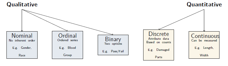
- Categorical variable (Qualitative)
- Numerical variable (Quantitative)
| Feature | Categorical Variable (Qualitative) | Numerical Variable (Quantitative) |
|---|---|---|
| Definition | Represents groups or categories that cannot be measured numerically | Represents quantitative values that can be measured and calculated |
| Data Type | Text or labels (sometimes coded as numbers) | Numbers (integers or decimals) |
| Examples | Gender (Male/Female), Eye color (Blue/Brown), Blood type (A/B/AB/O) | Age (25, 30), Height (170 cm), Salary ($5000) |
2.1.1 Types of Categorical (Qualitative) Variables
| Type | Definition | Examples |
|---|---|---|
| Nominal | Categories with no specific order | Colors: Red, Blue, Green; Blood type: A, B, AB, O |
| Ordinal | Categories with a specific order, but uneven differences between them | Ratings: Low, Medium, High; Education level: High School, Bachelor, Master |
| Dichotomous / Binary | Only two categories | Yes/No; Male/Female; Pass/Fail |
2.1.2 Types of Numerical (Quantitative) Variables
| Type | Definition | Examples |
|---|---|---|
| Interval | Continuous scale with equal gaps, but no true zero | Temperature in Celsius or Fahrenheit |
| Ratio | Continuous scale with equal gaps and a true zero | Height, Weight, Age, Salary |
A true zero means that the zero point on the scale represents the complete absence of the quantity being measured.
0°C does not mean “no temperature,” just a point on the scale. So it has no true zeros.
2.2 The Four Scales of Measurement
| Scale | Key Features | Notes / Examples |
|---|---|---|
| Nominal | - Two or more categories - No intrinsic order |
Examples: Gender (Male/Female), Blood type (A/B/AB/O) |
| Ordinal | - Two or more categories - Categories can be ordered/ranked - Magnitude between values not equal |
Examples: Education level (High School < Bachelor < Master), Ratings (Low, Medium, High) |
| Interval | - Measured on a continuous scale - No absolute zero - Differences between adjacent values are equal - Ratios not defined |
Examples: Temperature in Celsius or Fahrenheit |
| Ratio | - Interval variable with absolute zero - Ratios between values are defined |
Examples: Height, Weight, Age, Salary |
3. Summary Statistics
used in descriptive statistics, for
- summarize a set of observations
- communication information simply and quickly
3.1 Measure of Location (Central Tendency)
Tells us where the center or typical value of the data set lies
we use following to as main measurements in central tendency :
- Mean -> the average
- Median -> the middle value
- Mode -> the most frequent value
Example:
This tells us that the data is centered around 6.
3.1.1. Simple Arithmetic Mean
Notation:
- Mean of a population =
- Sample mean (when sample observations are known)=
- Sample mean (when sample observation is unknown)=
- Count of Numbers in the population = N
- Count of numbers in the sample = n
Given the population values:
Given a sample(values unknown):
Given a sample(values known):
3.1.2 Weighted Arithmetic Mean
Simple arithmetic gives equal importance to all the observations in a data set.
But when relative importance of the items in the distribution is not the same, we need to use this
Given
Exercise:
A student’s final marks in Mathematics, English, Statistics and Computer are 92, 76, 95, and 80 respectively. If the respective credits received for these courses are 2,
1, 3 and 4, determine an appropriate average mark.
3.1.3 Combined/Composite Arithmetic Mean
Simple arithmetic means of two or more related groups can be combined into a composite mean
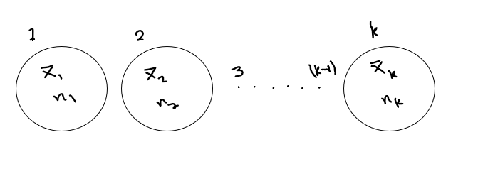
Given
Exercise:
There are three branches of a company, employing 100, 20, and 80 persons respectively. If the arithmetic means of the monthly salaries paid by the three
companies are Rs. 50000, 60000, and Rs. 80000 respectively, find the arithmetic mean
of the salaries of all the employees of the three companies.
3.1.4 Standard Geometric Mean (
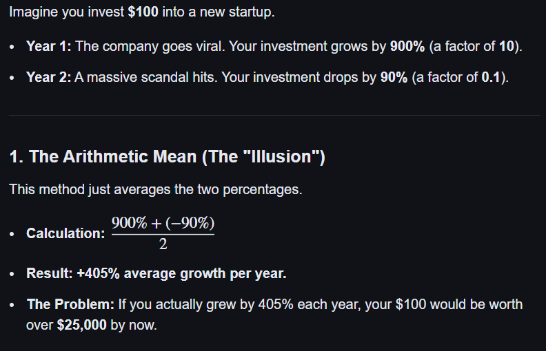
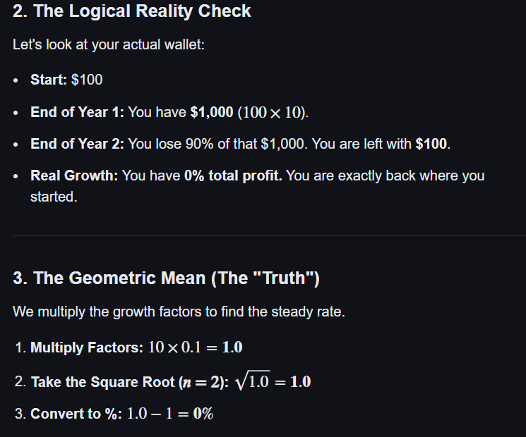
Primarily used to determine overall growth rates or averages of percentages over time
This can only be used in positive numbers
Used for a set of
Exercise:
The economic growth rate of a country for the last three years is 4%, 2%, and 8%. What is the overall growth rate?
-
Convert percentages to growth factors
-
Apply the geometric mean formula
- Multiply the values
- Take the cube root
- Convert back to a percentage growth rate
The overall economic growth rate over the three years is approximately 4.6%
3.1.5 Geometric Mean (An Alternative Version)
This version is used when dealing with growth rates that may include negative numbers (as long as they are greater than -1)
If the values are
Exercise:
The economic growth rate of a country for the last three years is 4%, -2%,
and 8%. What is the overall growth rate?
Three yearly growth rates: 4%, -2%, 8%
-
Convert to growth factors:
-
Multiply them:
-
Take the cubic root:
-
Convert to percentage:
The average yearly growth rate is 3.21%.
3.1.6 Harmonic Mean (

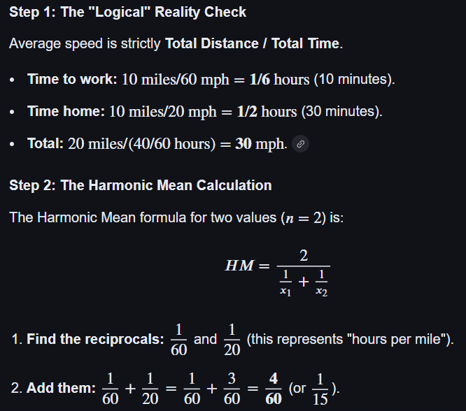
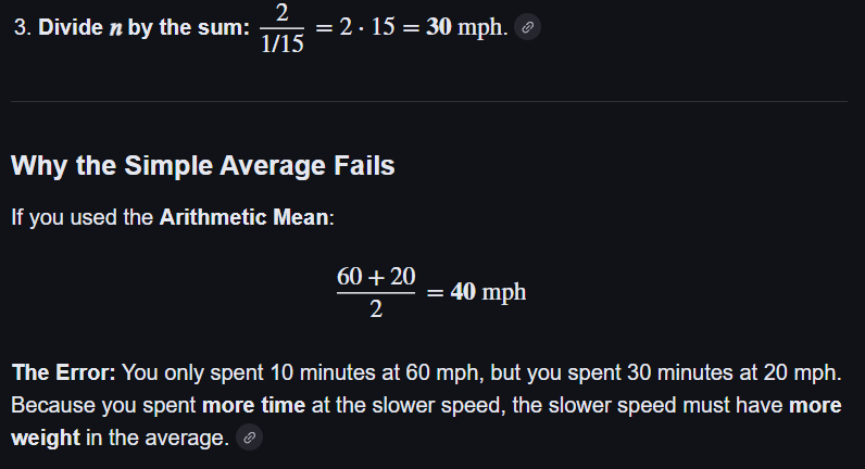
This is especially useful when dealing with rates or units, for example, calculating average speed.
For a set of
Where:
Exercise:
The speeds of three deliveries (in km per hour) of a fast bowler are 60, 90, and 100. What is the average speed?
- Write the harmonic mean formula
- Find the reciprocals
- Add the reciprocals
- Divide to find the harmonic mean
Final Answer
3.1.7 Relationship with Other Means
For any set of positive numbers with at least two different values, the following inequality holds:
Where:
This shows that the harmonic mean is always the smallest of the three averages.
Exercise:
Calculate the simple arithmetic mean, geometric mean, and harmonic mean
of 2, 4, 4, and 8.
- Conclusion
This confirms that the harmonic mean is the smallest, followed by the geometric mean, and the arithmetic mean is the largest.
3.1.8 Mode (Mo)
The mode is the value of a variable that occurs most frequently in a distribution.
Types of Mode:
- Unimodal: Only one mode in the series.
- Bimodal: Two modes in the series.
- Trimodal: Three modes in the series.
- Multimodal: More than three modes in the series.
Exercise:
12 students in a class have the following shoe sizes. What is the mode?
- Count the frequency of each value
| Shoe Size | Frequency |
|---|---|
| 6 | 1 |
| 7 | 1 |
| 8 | 5 |
| 9 | 3 |
| 10 | 2 |
-
Identify the mode
- The mode is the value with the highest frequency.
- Here, 8 occurs 5 times, which is more than any other value.
3.1.9 Median (Md)
The median is the middle value of a data set after arranging the observations in ascending order.
Let
- Case 1: When
The median is the value at the
position.
- Case 2: When
The median lies between the two positions:
The median is the average of the values at these two positions.
Examples:
Example 1: Odd Number of Observations
The 3rd value is:
Example 2: Even Number of Observations
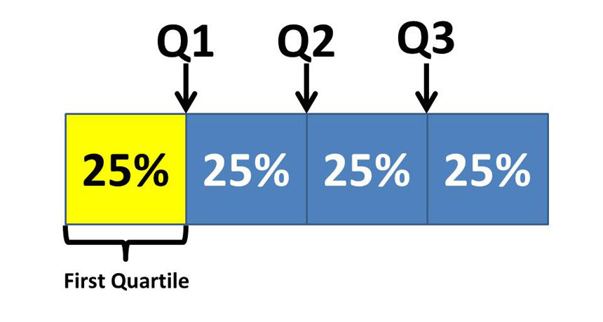
3.2 Quartiles (
Quartiles are values that divide an ordered data set into four equal parts.
Each part contains 25% of the total number of observations.
- (
- (
- (
Formula for the Location of Quartiles
Let (
Location of the
Exercise:
12 students in a class have the following weights (kg):
Find
- Arrange the data in ascending order
- Identify the number of observations
First Quartile
- Location
This lies between the 3rd and 4th items.
3rd item ( = 56 )
4th item ( = 59 )
- Value of
Second Quartile
- Location
This lies between the 6th and 7th items.
6th item ( = 67 )
7th item ( = 68 )
- Value of
Third Quartile
- Location
This lies between the 9th and 10th items.
9th item ( = 79 )
10th item ( = 81 )
- Value of
Interpretation
- 25% of students weigh less than 56.75 kg
- 50% of students weigh less than 67.5 kg
- 75% of students weigh less than 80.5 kg
Advantages and Disadvantages of Mean, Median, and Mode
| Measure | Advantages | Disadvantages |
|---|---|---|
| Mean | - Can be used with interval and ratio data - Has useful statistical properties (e.g., for variance, standard deviation) - Easy to understand and interpret |
- Affected by extreme values (outliers) - May not appear in the actual data - Requires interval/ratio scale data - Works best with symmetric distributions |
| Median | - Can be used with ordinal data - Unaffected by extreme values - Easy to calculate - Symmetric data not required |
- Restricted statistical uses - May not appear in the actual data |
| Mode | - Can be used with nominal data - Easy to calculate |
- Restricted statistical uses - Limited use for analysis |
3.3 Grouped Data Distributions
When dealing with large masses of raw data, it is often convenient to classify the data into groups or classes.
- **Frequency
- Grouped data distribution: A table showing classes and their corresponding frequencies.
Example Table – Weights of 600 University Students
| Class | Frequency |
|---|---|
| 30 - 39 | 7 |
| 40 - 49 | 126 |
| 50 - 59 | 278 |
| 60 - 69 | 123 |
| 70 - 79 | 62 |
| 80 - 89 | 4 |
3.3.1 Class Interval and Class Limits
- Class Interval: A symbol defining a class (e.g., 40–49).
- Class Limits: The smallest and largest numbers in a class:
- Lower Class Limit (LCL): Smaller number (e.g., 40)
- Upper Class Limit (UCL): Larger number (e.g., 49)
- Open Class Interval: A class that has no lower or upper limit indicated.
3.3.2 Class Boundaries / True class limits
If measurements are recorded to the nearest unit:
- The interval 40–49 includes all values from 39.5 to 49.5.
- Lower Class Boundary (LCB): 39.5
- Upper Class Boundary (UCB): 49.5
| Class | Frequency |
|---|---|
| 30 - 39 | 7 |
| 40 - 49 | 126 |
| 50 - 59 | 278 |
| 60 - 69 | 123 |
| 70 - 79 | 62 |
| 80 - 89 | 4 |
| Classes with Class Boundaries | Frequency |
|---|---|
| 29.5 - 39.5 | 7 |
| 39.5 - 49.5 | 126 |
| 49.5 - 59.5 | 278 |
| 59.5 - 69.5 | 123 |
| 69.5 - 79.5 | 62 |
| 79.5 - 89.5 | 4 |
3.3.3 Size (Width) of a Class Interval (
- Class Width : Difference between UCB and LCB.
- If all intervals have the same width, the common width is ( C ).
3.3.4 Class Mark / Midpoint (
- The midpoint of a class interval, used as the average of all observations in the class (assuming even distribution).
- Example: For class 40–49:
Summary Table for Example Data
| Class | LCL | UCL | LCB | UCB | Width ( C ) | Midpoint ( |
Frequency ( |
|---|---|---|---|---|---|---|---|
| 30–39 | 30 | 39 | 29.5 | 39.5 | 10 | 34.5 | 7 |
| 40–49 | 40 | 49 | 39.5 | 49.5 | 10 | 44.5 | 126 |
| 50–59 | 50 | 59 | 49.5 | 59.5 | 10 | 54.5 | 278 |
| 60–69 | 60 | 69 | 59.5 | 69.5 | 10 | 64.5 | 123 |
| 70–79 | 70 | 79 | 69.5 | 79.5 | 10 | 74.5 | 62 |
| 80–89 | 80 | 89 | 79.5 | 89.5 | 10 | 84.5 | 4 |
3.4 Measures of Central Tendency for Grouped Data
For grouped data, we calculate Mean, Mode, Median, Quartiles, Deciles, and Percentiles using class midpoints, class frequencies, and cumulative frequencies.
3.4.1 Mean (
Let (
and (
The mean is:
Example Table:
| Class | Frequency ( |
Midpoint ( |
|
|---|---|---|---|
| 30–39 | 7 | 34.5 | 241.5 |
| 40–49 | 126 | 44.5 | 5607 |
| 50–59 | 278 | 54.5 | 15151 |
| 60–69 | 123 | 64.5 | 7923.5 |
| 70–79 | 62 | 74.5 | 4619 |
| 80–89 | 4 | 84.5 | 338 |
3.4.2 Mode (
The mode is the value that occurs most frequently. For grouped data, the modal class has the highest frequency.
Where:
- (
- (
- (
- (
- (
- (
Example Table:
| Class | Frequency ( |
|---|---|
| 30–39 | 7 |
| 40–49 | 126 |
| 50–59 | 278 (modal) |
| 60–69 | 123 |
| 70–79 | 62 |
| 80–89 | 4 |
- The modal class = 50–59 (highest frequency = 278)
- Identify Required Values
| Symbol | Value |
|---|---|
| ( |
49.5 (lower boundary of modal class) |
| ( |
278 (frequency of modal class) |
| ( |
126 (frequency of class before modal class) |
| ( |
123 (frequency of class after modal class) |
| ( |
10 (class width) |
- Use the Modal Class Formula
Substitute the values:
- Simplify
3.4.3 Quartiles (
- Find cumulative frequencies.
- Use the formula for the
Where:
- (
- (
- (
- (
- (
Example Table:
| Class | Frequency ( |
|---|---|
| 30–39 | 7 |
| 40–49 | 126 |
| 50–59 | 278 |
| 60–69 | 123 |
| 70–79 | 62 |
| 80–89 | 4 |
- Calculate Cumulative Frequency (
| Class | ( |
Cumulative Frequency ( |
|---|---|---|
| 30–39 | 7 | 7 |
| 40–49 | 126 | 133 |
| 50–59 | 278 | 411 |
| 60–69 | 123 | 534 |
| 70–79 | 62 | 596 |
| 80–89 | 4 | 600 |
-
Calculate (
- (
- Locate quartile class: 50–59 (CF before = 133, f = 278, LCB = 49.5, C = 10)
- (
-
Calculate (
- (
- Quartile class = 50–59 (CF before = 133, f = 278, LCB = 49.5, C = 10)
- (
-
Calculate (
- (
- Quartile class = 60–69 (CF before = 411, f = 123, LCB = 59.5, C = 10)
- (
| Quartile | Value (kg) |
|---|---|
| 50.11 | |
| 55.51 | |
| 62.67 |
- 25% of students weigh less than 50.11 kg
- 50% of students weigh less than 55.51 kg
- 75% of students weigh less than 62.67 kg
3.4.4 Deciles (
Deciles are measures of position that divide a data set into 10 equal parts.
- Each part contains 10% of the total observations
- There are 9 deciles: (

Meaning of Each Decile
| Decile | Interpretation |
|---|---|
| ( |
10% of data lie below this value |
| ( |
20% of data lie below this value |
| ( |
30% of data lie below this value |
| ( |
40% of data lie below this value |
| ( |
50% of data lie below this value (Median) |
| ( |
60% of data lie below this value |
| ( |
70% of data lie below this value |
| ( |
80% of data lie below this value |
| ( |
90% of data lie below this value |
- Find cumulative frequencies.
- Use the formula for the
Where:
- (
- (
- (
- (
Example Table:
| Class | Frequency ( |
Cumulative Frequency ( |
|---|---|---|
| 30–39 | 7 | 7 |
| 40–49 | 126 | 133 |
| 50–59 | 278 | 411 |
| 60–69 | 123 | 534 |
| 70–79 | 62 | 596 |
| 80–89 | 4 | 600 |
Total number of observations:
Example – Find the 4th Decile (
- Locate the Decile Position
The value 240 lies in the class 50–59, since:
- CF before = 133
- CF of class = 411
So, the decile class is 50–59.
- Identify Required Values
| Symbol | Value |
|---|---|
| ( |
49.5 |
| ( |
133 |
| ( f |
278 |
| ( |
10 |
- Substitute into the Formula
- Simplify
3.4.5 Percentiles (
Percentiles are measures of position that divide a data set into 100 equal parts.
- Each part contains 1% of the total observations
- There are 99 percentiles: (
Meaning of Percentiles
| Percentile | Interpretation |
|---|---|
| ( |
10% of data lie below this value |
| ( |
25% of data lie below this value ( |
| ( |
50% of data lie below this value (Median) |
| ( |
75% of data lie below this value ( |
| ( |
90% of data lie below this value |
- Relation to Other Measures
When Percentiles Are Used
- To compare individual positions in large datasets
- Widely used in exam results, income distributions, and rankings
- Useful when data size is large and grouped
- Find cumulative frequencies.
- Use the formula for the
Where:
- (
- (
- (
- (
Example Table:
| Class (kg) | Frequency ( |
Cumulative Frequency ( |
|---|---|---|
| 30–39 | 7 | 7 |
| 40–49 | 126 | 133 |
| 50–59 | 278 | 411 |
| 60–69 | 123 | 534 |
| 70–79 | 62 | 596 |
| 80–89 | 4 | 600 |
Total number of observations:
Example: Find the 75th Percentile (
- Locate the Percentile Position
The value 450 lies in the class 60–69, since:
- CF before = 411
- CF of class = 534
So, the percentile class is 60–69.
- Identify Required Values
| Symbol | Value |
|---|---|
| ( |
59.5 |
| ( |
411 |
| ( |
123 |
| ( |
10 |
- Substitute into the Formula
- Simplify
3.5 Measures of Dispersion
Measures of dispersion describe how spread out the data values are around a central value.
They help us understand variability, consistency, and stability of data.
Common Measures of Dispersion
3.5.1 Range
The range is the simplest measure of dispersion.
It shows the difference between the largest and smallest values.
Example:
Data:
3.5.2 Interquartile Range (IQR)
The interquartile range measures the spread of the middle 50% of data.
Example:
Given:
3.5.3 Semi-Interquartile Range (SIQR)
The semi-interquartile range is half of the interquartile range.
Example:
3.5.4 Mean Deviation (MD)
Mean deviation measures the average deviation of values from the mean.
⚠️ Positive and negative deviations may cancel out.
Example:
Given Data
- Find the Mean
- Find Deviations from the Mean
| ( |
( |
|---|---|
| 2 | (2 - 4 = -2) |
| 4 | (4 - 4 = 0) |
| 6 | (6 - 4 = +2) |
- Apply the Mean Deviation Formula
⚠️ Important Observation
Although the data values are spread out, the mean deviation is zero because:
- Positive deviations cancel negative deviations
- This is why mean deviation is rarely used in practice
To avoid this cancellation problem, we use:
- Mean Absolute Deviation (MAD)
- Variance
- Standard Deviation
3.5.5 Mean Absolute Deviation (MAD)
Mean absolute deviation removes the sign by using absolute values.
Example:
Data:
Mean:
3.5.6 Median Absolute Deviation
This measure calculates deviation from the median.
Used when data contains outliers.
Example:
data:
- Arrange the Data
- Find the Median
The middle value is:
- Find Absolute Deviations from the Median
| Deviation from Median | |
|---|---|
| 2 | |
| 4 | |
| 5 | |
| 6 | |
| 100 |
- Apply the Formula
3.5.7 Variance
Variance measures how far data values spread around the mean.
Population Variance
Let (
Alternative form:
Sample Variance
For sample data:
When values are unknown
When values are known
Alternative form:
3.5.8 Standard Deviation
The standard deviation is the square root of variance.
It has the same unit as the original data.
It describes how far data values typically spread from the mean.
Sensitive to extreme values (outliers)
Population Standard Deviation
Sample Standard Deviation
When values are unknown
When values are known
Example:
If:
Then:
Interpretation
- Small standard deviation → data values are close to the mean
- Large standard deviation → data values are widely spread
3.5.9 Coefficient of Variation (CV)
The coefficient of variation compares relative variability between datasets.
Interpretation
- Higher CV → More variability, less consistency , less stability
- Lower CV → Less variability, more consistency , more stability
Example:
3.5.10 Variance for Grouped Data
For grouped data with class midpoints (
Where:
Example :
| Class Interval | ||
|---|---|---|
| 10–19 | 5 | 14.5 |
| 20–29 | 8 | 24.5 |
| 30–39 | 7 | 34.5 |
- Total Frequency
- Mean of Grouped Data
| 5 | 14.5 | 72.5 |
| 8 | 24.5 | 196 |
| 7 | 34.5 | 241.5 |
- Compute
| 14.5 | ( -11 ) | 121 |
| 24.5 | ( -1 ) | 1 |
| 34.5 | ( 9 ) | 81 |
- Multiply by Frequencies
| 5 | 121 | 605 |
| 8 | 1 | 8 |
| 7 | 81 | 567 |
- Variance